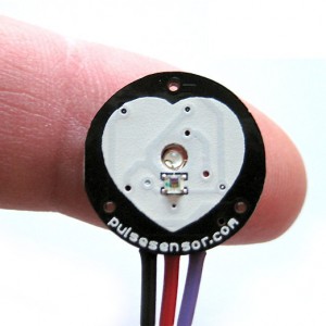
In this article outlined analysis of heart rate signals. A heart rate signal is obtained from the pulsesensor sensor.
This Sensor has been discussed in some of the previous articles:
The addition of this article is a filtering with LPF to help smooth the signal of the sensor results.
The signal processing stage is as follows:
- Pulsesensor as a source of signal coming from the heartbeat
- The voltage signal from the sensor is inserted into the resistor Filter and the capacitor as a low pass filter to avoid aliasing,
- The filter result voltage is inserted into the Arduino Nano module to be converted to digital with ADC. Data sampled with 1 kHz frequency with ADC on the Arduino Nano,
- Digital Data is then transmitted by asynchronous serial communication at a speed of 115200 bps through the USB port to the PC desktop.
- Data recorded on desktop PC with RealTerm software. Data is recorded to a TXT file on the PC.
- Record result Data is then analyzed with Python software using Jupyter Notebook
The software for the data measurements on the Arduino is as follows: https://github.com/waskita/embedded/tree/master/atmega-detak-jantung-profiling
The software for the analysis of signals is as follows: https://github.com/waskita/embedded/blob/master/analisis-detak-jantung/heart-beat-analysis-1kHz.ipynb
Here’s a signal flow block diagram on this system:

Here is details of the signal flow description of the system


The purpose of the sensor is to measure one’s heart rate.
There are a few things that complicate heart rate calculations:
- The amplitude of the signal varies depending on the hand condition, pressure on the sensor, and so on, so the signal threshold
- The heart rate signal has a high peak, and there are also smaller peaks. There must be an algorithm to detect high peaks only.
The ADC signal measurement results are still less flat, so to make the smoother filtering carried out at a frequency cut off of 4 Hz. The cut-off frequency of 4 Hz is selected considering the maximum heart rate of a normal person is 220 per minute, or equivalent to 3.667 Hz. So the signal above the frequency 3.667 Hz is not required.
Filter using a digital filter of IIR 4 pole. The 6 pole filter produces an unstable filter, and finally 4 pole is used. IIR filter types so that calculations are simpler, since this system will be implemented on microcontrollers with limited computing capabilities.
Design filter using Iowa Hills IIR Filter Designer Version 6.5 as follows:
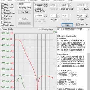
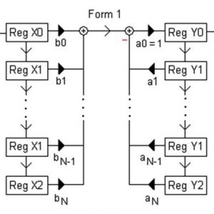
Implementation of filters with Python language, using the filter structure “Nth Order Coeffiecients”.
The structure of the IIR (Infinite Impulse Response) filter used is as follows:
The filter result is as follows (red signal).

The measurement Hasi signal contains a DC signal offset, so the average is not 0. To eliminate the DC offset, is done filtering with LPF at 200 mHz. Filter 2 pole IIR.
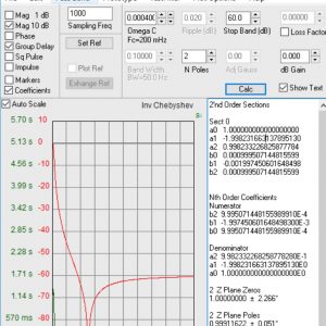
The filter results are as follows (red signal):

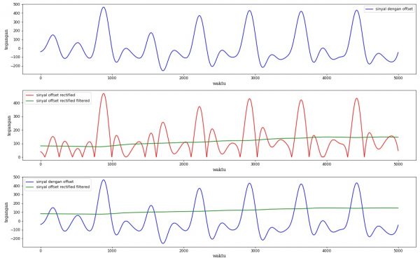
Signal without offset is obtained with the filter result signal 4 Hz reduced by the filter result signal at 0.2 Hz. The result is a signal (blue color) in the image below.
The blue signal is then seared (rectified), so there is a red signal.

The redirect signal is filtered again with the 0.2 Hz filter, to help peak detection. Peak detection is somewhat difficult, because of the 4 Hz filter results There is still a small peak. With the signal of a referral result is expected to detect high peaks only.
The final process is peak detection. Only high peaks are counted.

Cover
From experiments made, analog and digital filtering can help shape the signal so that it is easier to process.
