Juli 2023 – Elektrologi

Perancangan Filter

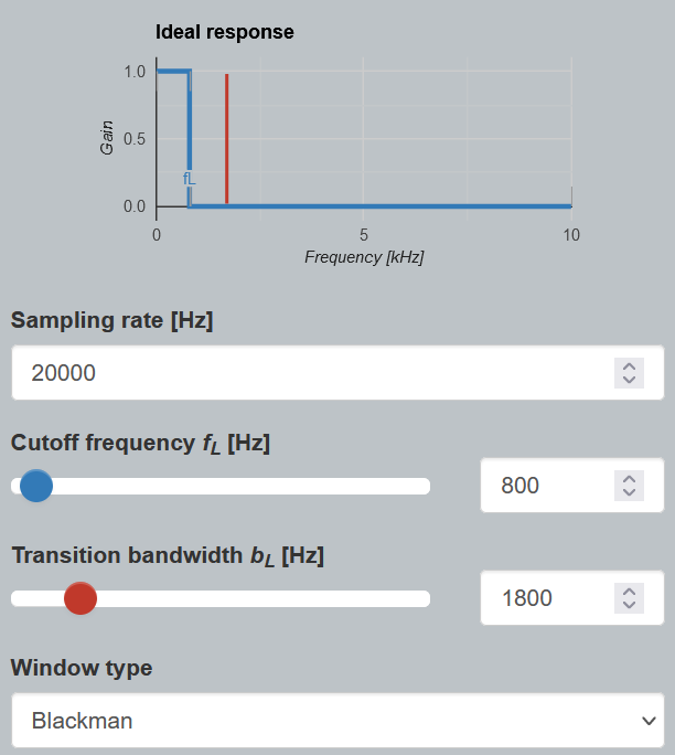
Perancangan filter menggunakan tools dari https://fiiir.com/

Parameter yang digunakan:

Sampling rate: 20000 Hz
Cut off frequency 800 Hz
Transition bandwidth 1800 Hz
Window type : Blackman

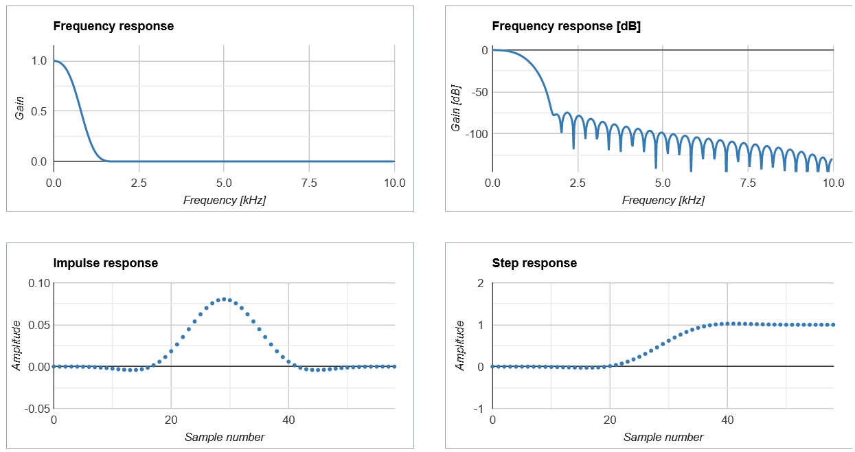
Berikut ini karakteristik filter yang dapat dilihat di laman yang sama

Kode dalam bahasa Python untuk menghitung parameter filter dan konvolusinya juga dihasilkan dari laman yang sama, sebagai berikut:

from __future__ import print_function
from __future__ import division

import numpy as np

# Example code, computes the coefficients of a low-pass windowed-sinc filter.

# Configuration.
fS = 20000 # Sampling rate.
fL = 800 # Cutoff frequency.
N = 53 # Filter length, must be odd.

# Compute sinc filter.
h = np.sinc(2 * fL / fS * (np.arange(N) - (N - 1) / 2))

# Apply window.
h *= np.blackman(N)

# Normalize to get unity gain.
h /= np.sum(h)

print(h)

# Applying the filter to a signal s can be as simple as writing
# s = np.convolve(s, h)

Parameter filter yang dihasilkan adalah sebagai berikut (sebagai Python array)

[-4.29317419e-20 -4.18549678e-21 -1.79819385e-05 -8.38178513e-05
 -2.28616892e-04 -4.79528638e-04 -8.51847897e-04 -1.33864303e-03
 -1.89910369e-03 -2.44776137e-03 -2.84740649e-03 -2.90866942e-03
 -2.39870072e-03 -1.06016948e-03  1.35995551e-03  5.07437980e-03
  1.02166209e-02  1.68050560e-02  2.47160945e-02  3.36720917e-02
  4.32479500e-02  5.28978134e-02  6.20002342e-02  6.99171799e-02
  7.60597872e-02  7.99523091e-02  8.12855501e-02  7.99523091e-02
  7.60597872e-02  6.99171799e-02  6.20002342e-02  5.28978134e-02
  4.32479500e-02  3.36720917e-02  2.47160945e-02  1.68050560e-02
  1.02166209e-02  5.07437980e-03  1.35995551e-03 -1.06016948e-03
 -2.39870072e-03 -2.90866942e-03 -2.84740649e-03 -2.44776137e-03
 -1.89910369e-03 -1.33864303e-03 -8.51847897e-04 -4.79528638e-04
 -2.28616892e-04 -8.38178513e-05 -1.79819385e-05 -4.18549678e-21
 -4.29317419e-20]

Simulasi dengan Python di Desktop

Berikut ini kode untuk simulasi filter tersebut di Jupyter Notebook dengan bahasa Python.

from __future__ import print_function
from __future__ import division

import numpy as np
import math
import matplotlib.pyplot as plt

# Example code, computes the coefficients of a low-pass windowed-sinc filter.

# Configuration.
fS = 20000 # Sampling rate.
fL = 800 # Cutoff frequency.
N = 53 # Filter length, must be odd.

# Compute sinc filter.
h = np.sinc(2 * fL / fS * (np.arange(N) - (N - 1) / 2))

# Apply window.
h *= np.blackman(N)

# Normalize to get unity gain.
h /= np.sum(h)

print(h)

# Applying the filter to a signal s can be as simple as writing
# s = np.convolve(s, h)

x = np.linspace(0,1, 20001)

# filter digital
signal_frequency=8000 # diubah-ubah sesuai keperluan
y=np.sin(x*2*math.pi * signal_frequency)
# Applying the filter to a signal s can be as simple as writing
y_out = np.convolve(y, h)
plt.figure(figsize=(16,6))
plt.plot(x, y_out[0:20001],label="output")
plt.plot(x, y[0:20001],label="input")
plt.title("signal:{} Hz".format(signal_frequency))
plt.legend()
plt.axis('tight')
plt.xlim([0, 0.01])
plt.savefig("simulasi-signal-{}.jpg".format(signal_frequency))

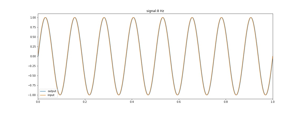
Hasil simulasi untuk frekuensi 8 Hz

Hasil simulasi untuk frekuensi 80 HzHasil simulasi untuk frekuensi 800 Hz

Hasil simulasi untuk frekuensi 8000 Hz

Simulasi dengan C di Desktop

Pada percobaan ini filter disimulasikan di Desktop PC untuk mengecek ketepatan perhitungan dibandingkan dengan versi Python.

Kode untuk simulasi C sebagai berikut:

#include <stdio.h>
#include <stdlib.h>
#include "math.h"

int main()
{

#define ORDE_FILTER 53
int i,j,k;
FILE * fp;
char filename[100];
printf("Hello world!\n");
// simulasi 1 detik saja

float signal_frequency=8; // frekuensi input signal
float filter_coefficients[]= {-4.29317419e-20, -4.18549678e-21, -1.79819385e-05, -8.38178513e-05,
-2.28616892e-04, -4.79528638e-04, -8.51847897e-04, -1.33864303e-03,
-1.89910369e-03, -2.44776137e-03, -2.84740649e-03, -2.90866942e-03,
-2.39870072e-03, -1.06016948e-03, 1.35995551e-03, 5.07437980e-03,
1.02166209e-02, 1.68050560e-02, 2.47160945e-02, 3.36720917e-02,
4.32479500e-02, 5.28978134e-02, 6.20002342e-02, 6.99171799e-02,
7.60597872e-02, 7.99523091e-02, 8.12855501e-02, 7.99523091e-02,
7.60597872e-02, 6.99171799e-02, 6.20002342e-02, 5.28978134e-02,
4.32479500e-02, 3.36720917e-02, 2.47160945e-02, 1.68050560e-02,
1.02166209e-02, 5.07437980e-03, 1.35995551e-03, -1.06016948e-03,
-2.39870072e-03, -2.90866942e-03, -2.84740649e-03, -2.44776137e-03,
-1.89910369e-03, -1.33864303e-03, -8.51847897e-04, -4.79528638e-04,
-2.28616892e-04, -8.38178513e-05, -1.79819385e-05, -4.18549678e-21,
-4.29317419e-20
};
int orde_filter=ORDE_FILTER;
float y_history[ORDE_FILTER];
signal_frequency=8000;
sprintf(filename,"simulasi-%d.csv",(int)signal_frequency);
fp = fopen (filename, "w");
fprintf(fp,"time,y,y_out\n");

// zeros y_history
for (i=0; i<orde_filter; i++)
{
y_history[i]=0;
}
for (i=0; i<20000; i++)
{
printf(".");
float t,y;
t=(float)i/(float)20000; // time axis
y=sin(2 * M_PI *signal_frequency* t);
// fprintf(fp,"%f,%f\n",t,y);

// hitung history signal
for (j=orde_filter-1; j>=1; j--)
{
int src=j-1;
int dst=j;
y_history[dst]=y_history[src];
// printf("%d %d\n",src,dst);
}
y_history[0]=y;

// hitung konvolusi
float y_out=0;
for (k=0; k<orde_filter; k++)
{
// fprintf(fp,"%5.3f ",y_history[k]);
y_out=y_out+y_history[k]*filter_coefficients[k];
}
// fprintf(fp,"\n");
fprintf(fp,"%f,%f,%f\n",t,y,y_out);
}
fclose(fp);
return 0;
}



// https://www.tutorialspoint.com/c_standard_library/c_function_fprintf.htm

Output kode C tersebut berupa file *.csv

Visualisasi data di file *.csv dilakukan menggunakan Jupyter Notebook dengan kode sebagai berikut:

import pandas as pd
import math
import matplotlib.pyplot as plt

name="simulasi-8"
name="simulasi-80"
name="simulasi-800"
name="simulasi-8000"
df = pd.read_csv('../filter-simulasi-c/{}.csv'.format(name))

plt.figure(figsize=(16,6))
plt.plot(df["time"], df["y"],marker='o',label="input")
plt.plot(df["time"], df["y_out"],marker='o',label="output")
plt.legend()
plt.axis('tight')
plt.xlim([0, 0.001])
plt.savefig("visualisasi-{}.jpg".format(name))

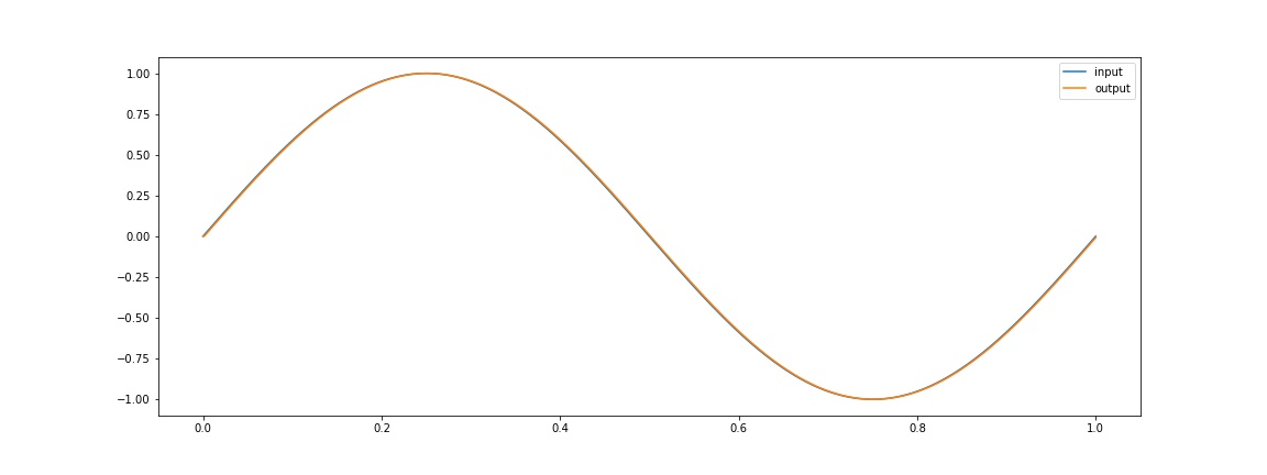
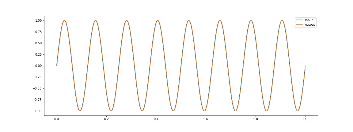
Tampilan Visualisasi untuk sinyal 8 Hz

nampak sinyal 8 Hz tidak teredam

Tampilan Visualisasi untuk sinyal 80 Hz

sinyal 80 Hz nampak teredam sedikit sekali dan ada lag

Tampilan Visualisasi untuk sinyal 800 Hz

nampak sinyal 800 Hz teredam sekitar 50%

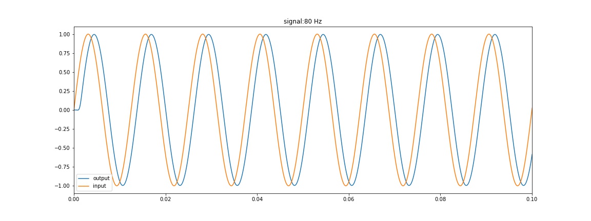
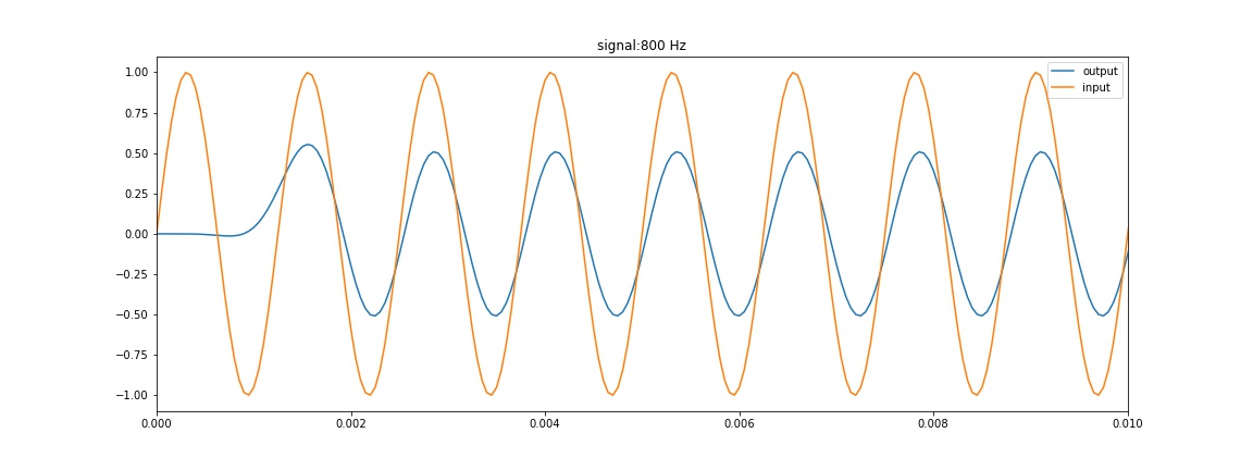
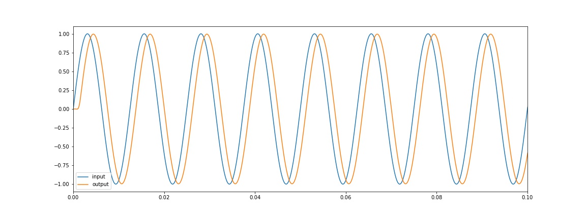
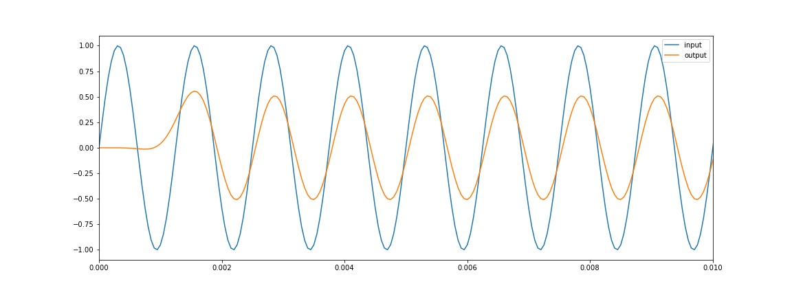
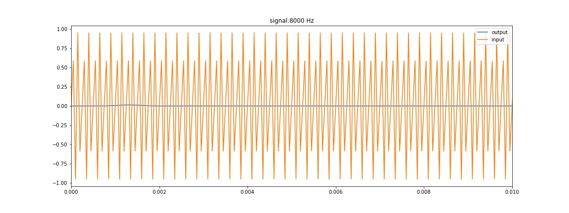
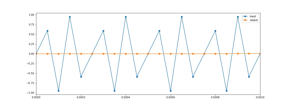
Tampilan Visualisasi untuk sinyal 8000 Hz

nampak sinyal 8000 Hz teredam hampir semuanya

Simulasi dengan C di ESP32

pada percobaan ini kode dijalankan di ESP32 namun input adalah simulasi bukan dari generator sinyal. Output direkam ke port serial, bukan ke osiloskop.

Kode ESP32 adalah sebagai berikut

#define ORDE_FILTER 53

void setup() {

  Serial.begin(115200);

  //

  int i, j, k;

  char filename[100];

  // simulasi 1 detik saja

  float signal_frequency = 8;  // frekuensi input signal

  float filter_coefficients[] = { -4.29317419e-20, -4.18549678e-21, -1.79819385e-05, -8.38178513e-05,

                                  -2.28616892e-04, -4.79528638e-04, -8.51847897e-04, -1.33864303e-03,

                                  -1.89910369e-03, -2.44776137e-03, -2.84740649e-03, -2.90866942e-03,

                                  -2.39870072e-03, -1.06016948e-03, 1.35995551e-03, 5.07437980e-03,

                                  1.02166209e-02, 1.68050560e-02, 2.47160945e-02, 3.36720917e-02,

                                  4.32479500e-02, 5.28978134e-02, 6.20002342e-02, 6.99171799e-02,

                                  7.60597872e-02, 7.99523091e-02, 8.12855501e-02, 7.99523091e-02,

                                  7.60597872e-02, 6.99171799e-02, 6.20002342e-02, 5.28978134e-02,

                                  4.32479500e-02, 3.36720917e-02, 2.47160945e-02, 1.68050560e-02,

                                  1.02166209e-02, 5.07437980e-03, 1.35995551e-03, -1.06016948e-03,

                                  -2.39870072e-03, -2.90866942e-03, -2.84740649e-03, -2.44776137e-03,

                                  -1.89910369e-03, -1.33864303e-03, -8.51847897e-04, -4.79528638e-04,

                                  -2.28616892e-04, -8.38178513e-05, -1.79819385e-05, -4.18549678e-21,

                                  -4.29317419e-20 };

  int orde_filter = ORDE_FILTER;

  float y_history[ORDE_FILTER];

  signal_frequency = 800;

//  signal_frequency = 80;

//  signal_frequency = 8;

  sprintf(filename, "simulasi-%d.csv", (int)signal_frequency);

  printf("time,y,y_out\n");

  // zeros y_history

  for (i = 0; i < orde_filter; i++) {

    y_history[i] = 0;

  }

  for (i = 0; i < 20000; i++) {

    float t, y;

    t = (float)i / (float)20000;  //  time axis

    y = sin(2 * M_PI * signal_frequency * t);

    //        fprintf(fp,"%f,%f\n",t,y);

    // hitung history signal

    for (j = orde_filter - 1; j >= 1; j--) {

      int src = j - 1;

      int dst = j;

      y_history[dst] = y_history[src];

      //            printf("%d %d\n",src,dst);

    }
   y_history[0] = y;
    // hitung konvolusi
    float y_out = 0;
    for (k = 0; k < orde_filter; k++) {
      y_out = y_out + y_history[k] * filter_coefficients[k];
    }

    //        fprintf(fp,"\n");

    printf("%f,%f,%f\n", t, y, y_out);

  }

}

void loop() {

  // put your main code here, to run repeatedly:

}

Output dari ESP32 direkam dengan software RealTerm ke sebuah file *.txt

File *.txt tersebut dirapikan dan disimpan sebagai *.csv

File *.csv ini kemudian divisualisasikan dengan Jupyter Notebook

Kode visualisasi sebagai berikut

# graph simulasi C filter
import pandas as pd
import math
import matplotlib.pyplot as plt

name="esp32-8.csv"
name="esp32-80.csv"
#name="esp32-800.csv"
#name="esp32-8000.csv"
df = pd.read_csv('{}'.format(name))

plt.figure(figsize=(16,6))
plt.plot(df["time"], df["y"],label="input")
plt.plot(df["time"], df["y_out"],label="output")
plt.legend()
plt.axis('tight')
plt.xlim([0, 0.1])
plt.title(name)
plt.savefig("visualisasi-{}.jpg".format(name))

Sinyal 8 Hz:

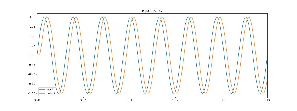
Sinyal 80 Hz

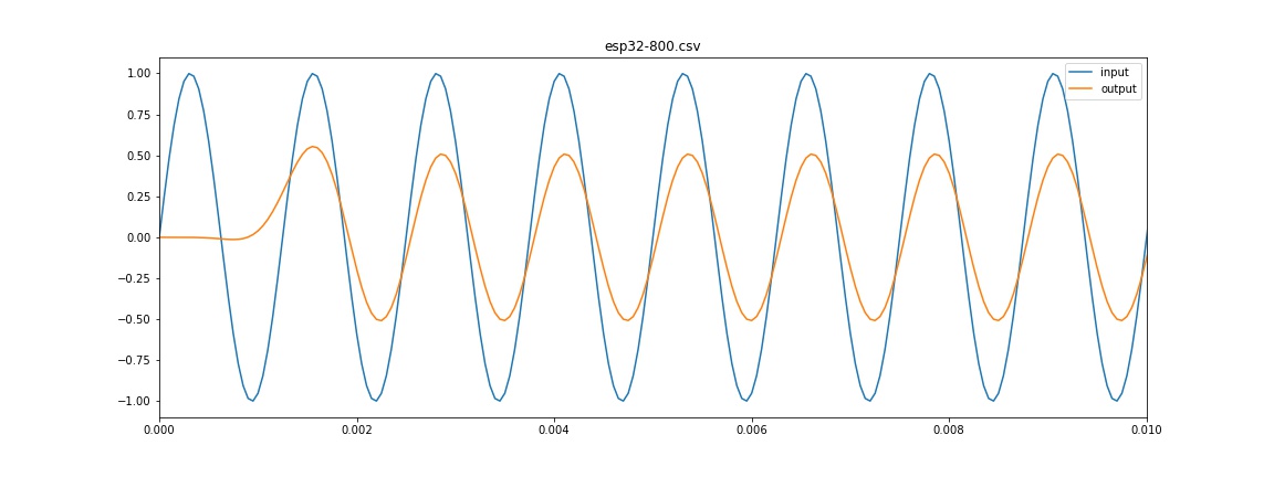
Sinyal 800 Hz

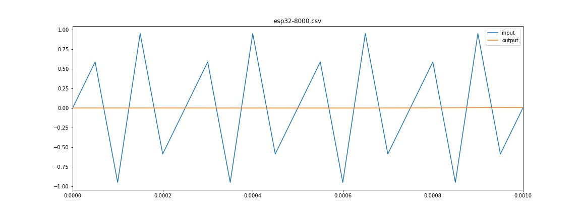
Sinyal 8000 Hz

Kesimpulan: output dari software LPF di ESP32 sama dengan output dari software C di Desktop

Profiling di ESP32

Pada percobaan ini waktu yang diperlukan untuk menghitung filter diukur di ESP32.

Pewaktuan menggunakan fungsi millis(). Fungsi millis() tidak 100% akurat. Untuk lebih tepat perlu interupsi timer, atau dengan osiloskop.

Kode profiling:

#define ORDE_FILTER 53

float buffer[100];

void setup() {

int buffer_index = 0;

int durasi;

Serial.begin(115200);

long int i;

int j, k;

char filename[100];

// simulasi 1 detik saja

float signal_frequency = 8; // frekuensi input signal

float filter_coefficients[] = { -4.29317419e-20, -4.18549678e-21, -1.79819385e-05, -8.38178513e-05,

-2.28616892e-04, -4.79528638e-04, -8.51847897e-04, -1.33864303e-03,

-1.89910369e-03, -2.44776137e-03, -2.84740649e-03, -2.90866942e-03,

-2.39870072e-03, -1.06016948e-03, 1.35995551e-03, 5.07437980e-03,

1.02166209e-02, 1.68050560e-02, 2.47160945e-02, 3.36720917e-02,

4.32479500e-02, 5.28978134e-02, 6.20002342e-02, 6.99171799e-02,

7.60597872e-02, 7.99523091e-02, 8.12855501e-02, 7.99523091e-02,

7.60597872e-02, 6.99171799e-02, 6.20002342e-02, 5.28978134e-02,

4.32479500e-02, 3.36720917e-02, 2.47160945e-02, 1.68050560e-02,

1.02166209e-02, 5.07437980e-03, 1.35995551e-03, -1.06016948e-03,

-2.39870072e-03, -2.90866942e-03, -2.84740649e-03, -2.44776137e-03,

-1.89910369e-03, -1.33864303e-03, -8.51847897e-04, -4.79528638e-04,

-2.28616892e-04, -8.38178513e-05, -1.79819385e-05, -4.18549678e-21,

-4.29317419e-20 };

int orde_filter = ORDE_FILTER;

float y_history[ORDE_FILTER];

signal_frequency = 800;

// signal_frequency = 80;

// signal_frequency = 8;

printf(“time,y,y_out\n”);

// zeros y_history

for (i = 0; i < orde_filter; i++) {

y_history[i] = 0;

}

int time_start = millis();

for (i = 0; i < 1000000L; i++) {

float t, y;

t = (float)i / (float)20000; // time axis

y = sin(2 * M_PI * signal_frequency * t);

// fprintf(fp,”%f,%f\n”,t,y);

// hitung history signal

for (j = orde_filter – 1; j >= 1; j–) {

int src = j – 1;

int dst = j;

y_history[dst] = y_history[src];

// printf(“%d %d\n”,src,dst);

}

y_history[0] = y;

// hitung konvolusi

float y_out = 0;

for (k = 0; k < orde_filter; k++) {

y_out = y_out + y_history[k] * filter_coefficients[k];

}

// fprintf(fp,”\n”);

// Serial.print(“.”);

buffer[buffer_index] = y_out;

buffer_index++;

if (buffer_index>100){

buffer_index=0;

}

int time_end = millis();

durasi = time_end – time_start;

Serial.println(“durasi”);

Serial.println(durasi);

}

void loop() {

// put your main code here, to run repeatedly:

}

Hasil profiling: kode memerlukan 16479 ms untuk menjalankan 1000000 kali perhitungan. jadi setiap perhitungan memerlukan 16.479 us

Konversi DAC di ESP32 memerlukan sekitar 20 us (pesimis), jadi jika kode sekuensial maka didapatkan perioda 36.479 us, atau frekuensi = 27413 Hz.

Frekuensi filter yang dirancang adalah 20000 Hz, jadi masih di bawah batas 27413 Hz.

Pengujian Dengan Sinyal Sesungguhnya

Pada percobaan ini kode dijalankan di ESP32 dengan input dari generator sinyal dan output diamati di osiloskop

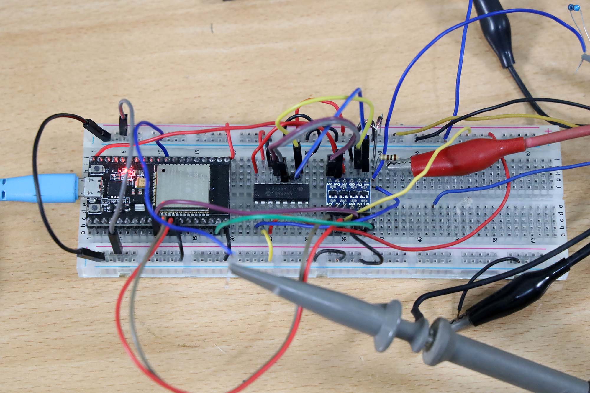
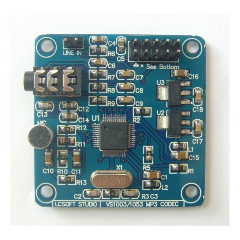
Berikut ini implementasi rangkaian:

Implementasi software dapat dilihat di https://github.com/waskita/embedded/tree/master/esp32_mcp3008_baker_adc_dac_filter-timer

Sinual input didapat dari generator sinyal GW Instek AFG-2012

Pengukuran output menggunakan osiloskop GW Instek-1152A-U

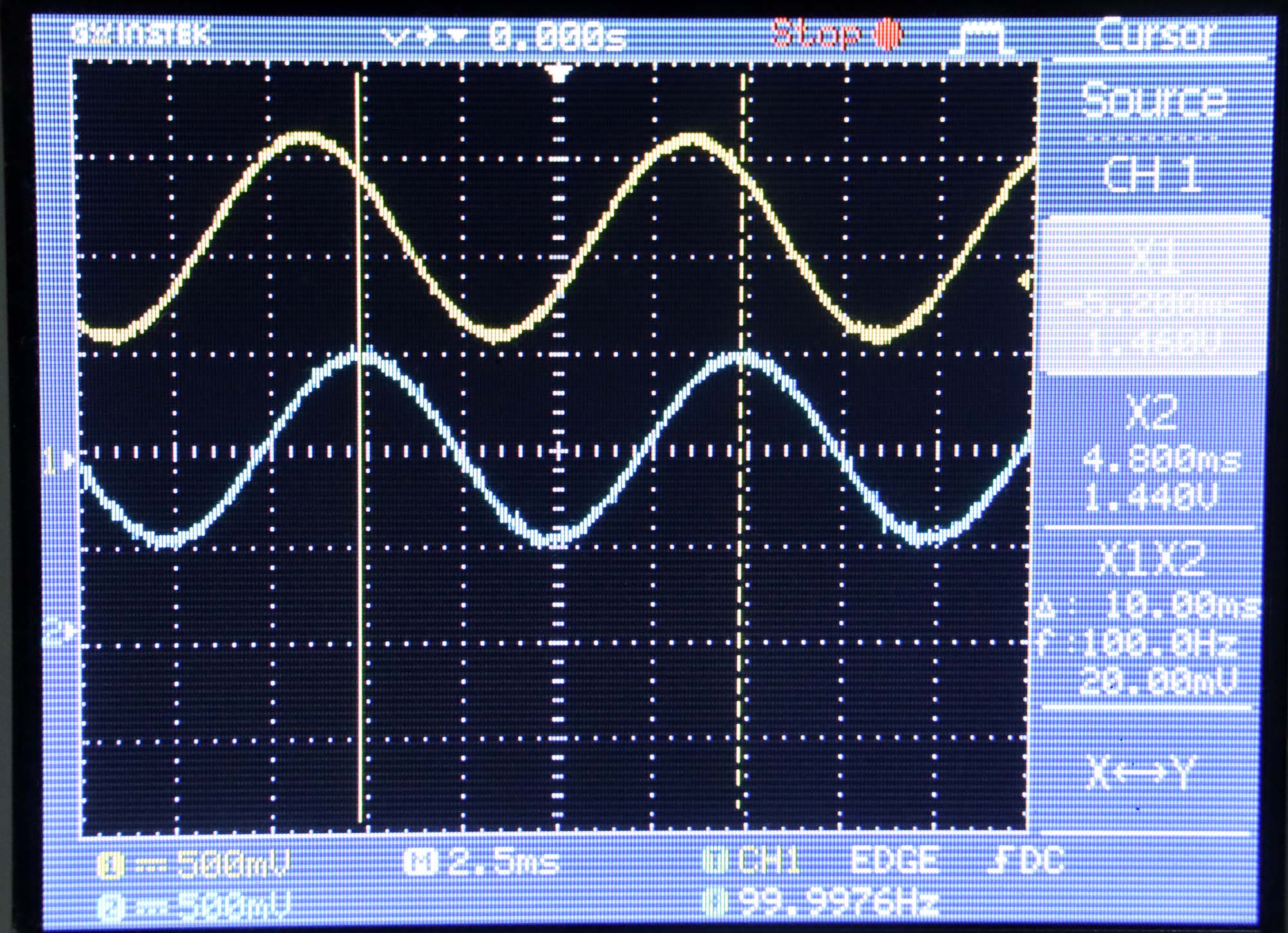
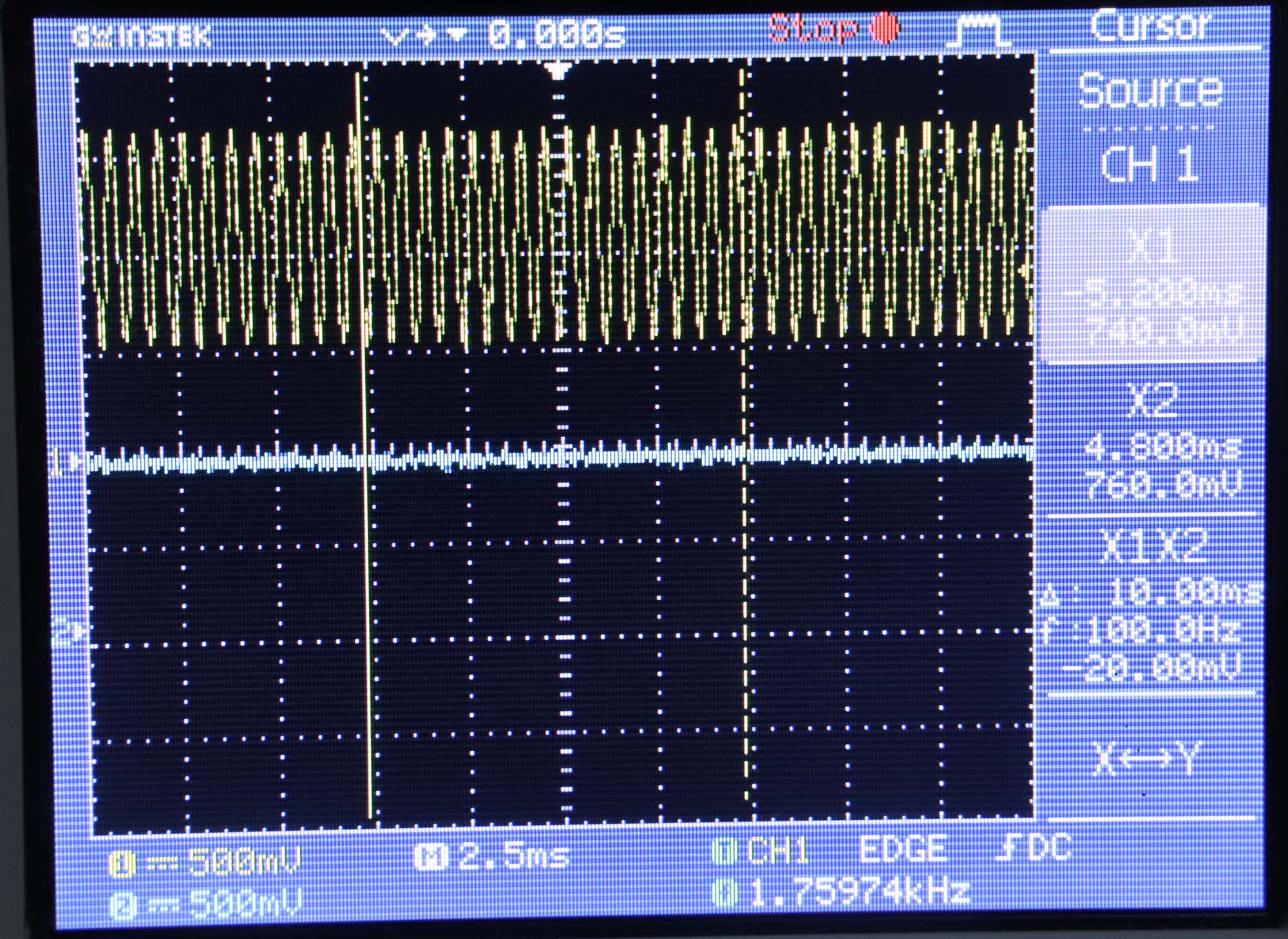
Berikut ini pengukuran pada frekuensi cut off = 100 Hz jauh di bawah frekuensi cut off.

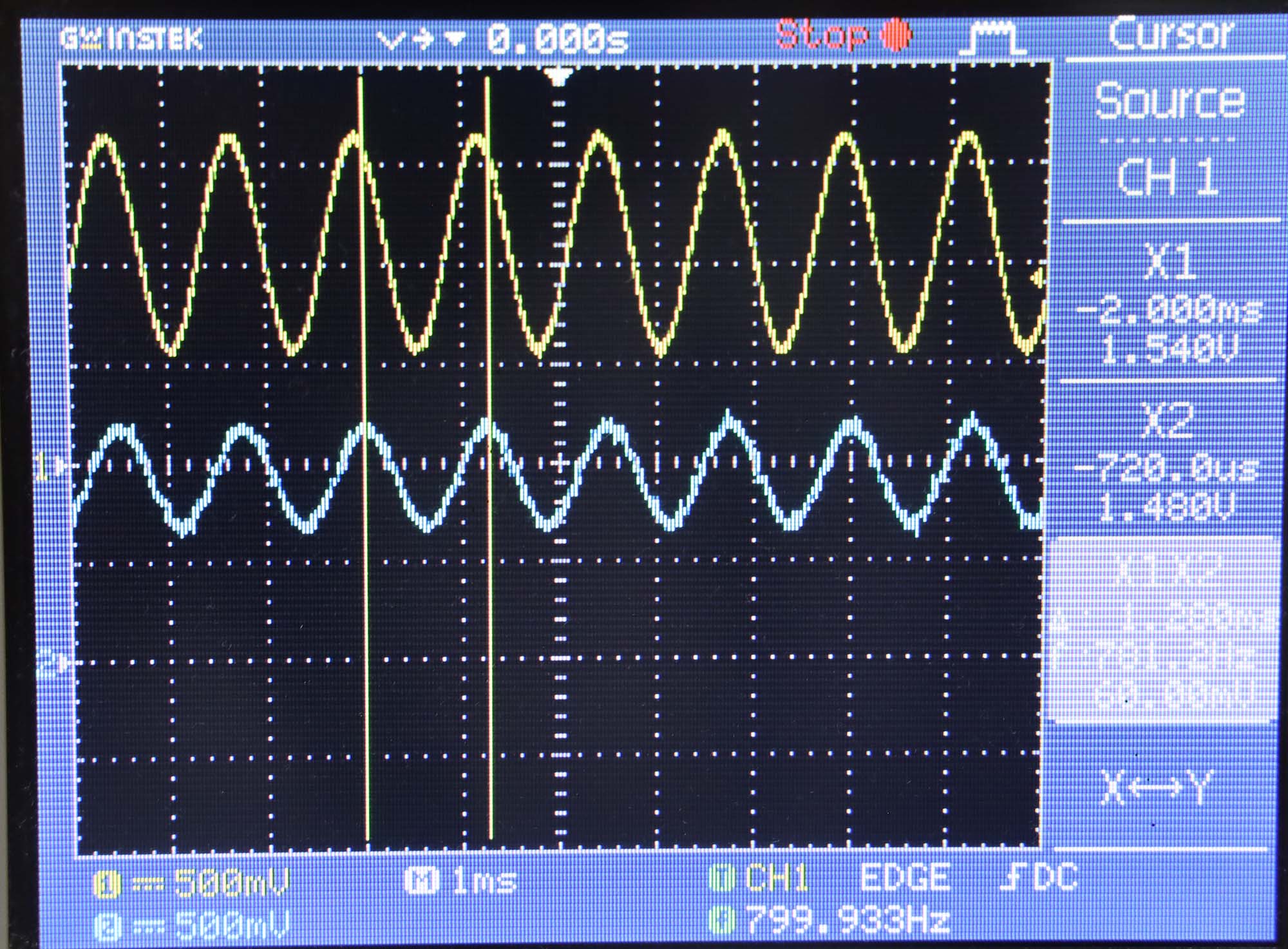
Berikut ini pengukuran pada frekuensi cut off = 800 Hz. Amplitudo sinyal output sekitar 50% sinyal input.

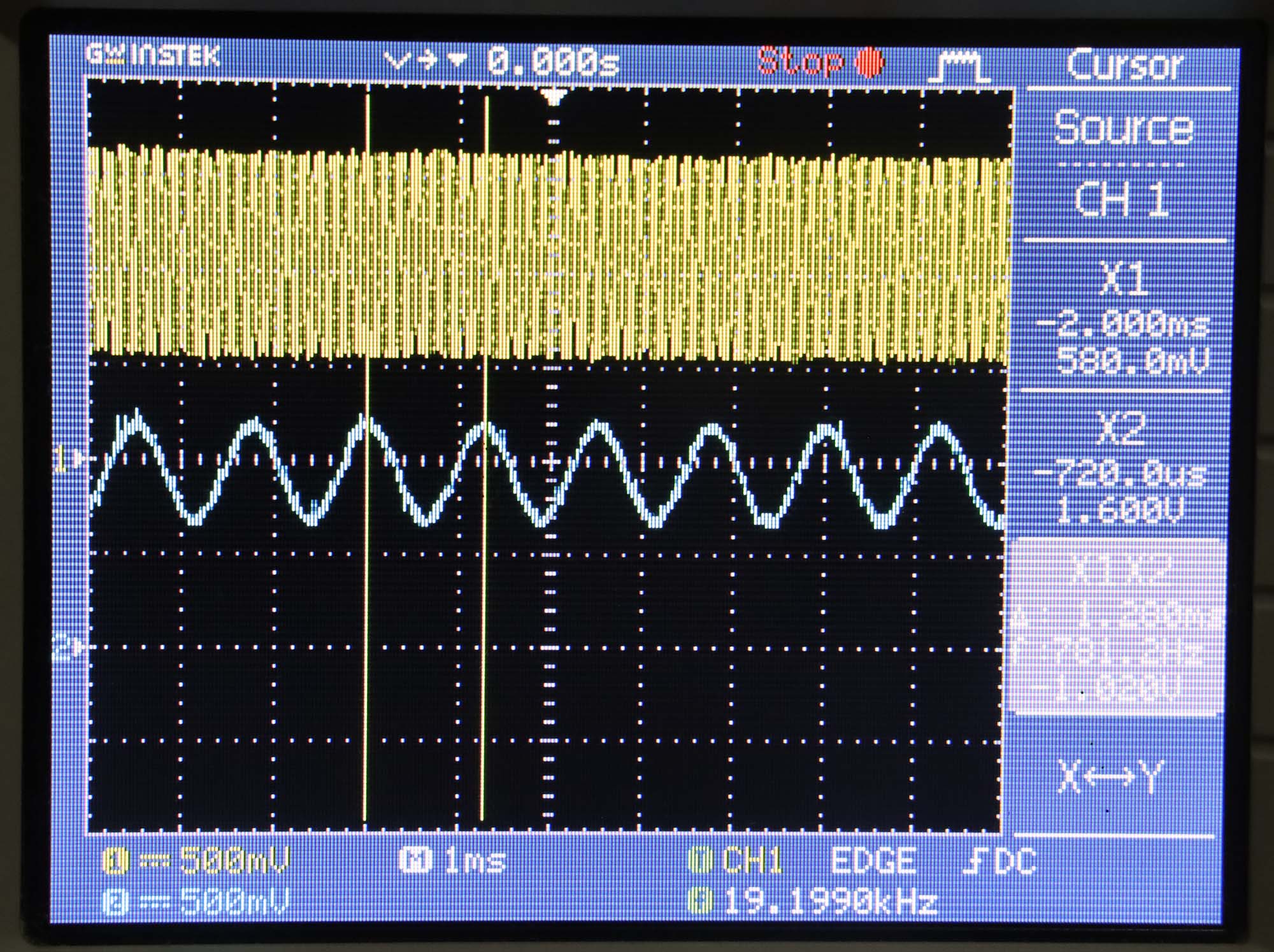
Berikut ini pengukuran pada frekuensi 1600 Hz, jauh di atas cut off. Amplitudo sinyal output kecil sekali hampir tidak ada.

Berikut ini pengukuran pada frekuensi input 19200 Hz. Terjadi aliasing karena pada sistem ini tidak ada filter anti aliasing.

Referensi

Design FIR & IIR Filters from Tom Roelandts

Bulan: Juli 2023

ADC dan DAC Populer

Literatur

Motor Driver RZ7889

Perancangan dan Implementasi Low Pass Filter Digital Dengan ESP32

Perancangan Filter

Simulasi dengan Python di Desktop

Simulasi dengan C di Desktop

Simulasi dengan C di ESP32

Profiling di ESP32

Pengujian Dengan Sinyal Sesungguhnya

Referensi

Modul Audio VS1053

Referensi